Preppin' Data - Introductory Month Solutions using Python

Data Preparation is one of the key tasks someone who works in Data must do, as most data sources are do not have the structure you really need for your analysis or your work. And I always asked myself: How can I learn Data Preparation? Once when scrolling through TikTok someone recommended the website Preppin' Data. So I took a look at it and got hooked.

But what is Preppin' Data? Preppin' Data is a blog and website which posts generally about Data Preparation and has weekly data preparation challenges in which you can solve. They focus mostly on data preparation using Tableau, which I haven't worked with yet. Since data preparation is not limited to Tableau of course, I will use Python to solve those challenges and I want to share my steps and solutions with you.

As of writing this article there are 15 challenges online since January this year and they are currently divided in Introductory Month, Intermediate Month and Advanced Month. I will start and combine the challenges for those months togehter in this and upcoming posts. Maybe if I feel like it, my solutions for the challenges afterwards will follow as well.

Week 1

The Challenge

The given data consists of a CSV-file containing transactions of the Data Source Bank (DSB) as well as transactions from other banks. Given were 5 columns: Transaction Code, Value, Customer Code, Online or In-Person and Transaction Date. The goal is now to transform some columns and sum the Value column in three different ways. For the complete challenge, please take a look at the original webpage here: https://preppindata.blogspot.com/2023/01/2023-week-1-data-source-bank.html.

The Solution

Since I'm already familiar with using pandas we can use that here. The first thing we do was to load the data into a pandas DataFrame using the read_csv function and then take a look at the initial data just to get familiar with how the data looks and feels.

import pandas as pd
df = pd.read_csv("PD 2023 Wk 1 Input.csv")
df.head()

The first task was the extraction of the bank code from the transaction code in the first column. As the data shows, the transaction code is always at the beginning of the data. From my perspective there are now two options: Either we go with a regular expression, which gets all letters from the transaction code, or we just split the string by using the "-" as a delimiter and take the first element from that resulting array as my bank code (which we do here).

df["Bank"] = df["Transaction Code"].apply(lambda x : x.split("-")[0])
df.head()

The second task was to replace the 1s and 2s in the Online or In-Person column with the corresponding text value, which should be quite easy using the replace function pandas Series objects.

df["Online or In-Person"] = df["Online or In-Person"].replace({1 : "Online", 2: "In-Person"})
df.head()

For turning the transaction date into the day name, we need to import the datetime library first to parse the date string from the given data into a datetime object. Here the strptime function comes in handy to do so. After that pandas gives us already the built-in option to get the day name from the datetime object directly:

import datetime
df["Transaction Date"] = df["Transaction Date"].apply(lambda x : datetime.datetime.strptime(x, "%d/%m/%Y %H:%M:%S"))
df["Transaction Date"] = df["Transaction Date"].dt.day_name()
df.head()

After the three transformation steps we now only need to aggregate the data in three different ways, using the pandas groupby function and output it as a CSV to get the files we want:

df[["Bank", "Value"]].groupby(["Bank"]).sum().reset_index().to_csv("ByBank.csv", index=False)
df[["Bank", "Transaction Date", "Online or In-Person", "Value"]].groupby(["Bank", "Transaction Date", "Online or In-Person"]).sum().reset_index().to_csv("ByBank_Transaction-Date_Type.csv", index=False)
df[["Bank", "Customer Code", "Value"]].groupby(["Bank", "Customer Code"]).sum().reset_index().to_csv("ByBank_CustomerCode.csv", index=False)

When combining all code pieces the complete code would look like this:

df = pd.read_csv("PD 2023 Wk 1 Input.csv")
df["Bank"] = df["Transaction Code"].apply(lambda x : x.split("-")[0])
df["Online or In-Person"] = df["Online or In-Person"].replace({1 : "Online", 2: "In-Person"})
df["Transaction Date"] = df["Transaction Date"].apply(lambda x : datetime.datetime.strptime(x, "%d/%m/%Y %H:%M:%S"))
df["Transaction Date"] = df["Transaction Date"].dt.day_name()
df[["Bank", "Value"]].groupby(["Bank"]).sum().reset_index().to_csv("ByBank.csv", index=False)
df[["Bank", "Transaction Date", "Online or In-Person", "Value"]].groupby(["Bank", "Transaction Date", "Online or In-Person"]).sum().reset_index().to_csv("ByBank_Transaction-Date_Type.csv", index=False)
df[["Bank", "Customer Code", "Value"]].groupby(["Bank", "Customer Code"]).sum().reset_index().to_csv("ByBank_CustomerCode.csv", index=False)

Week 2

The Challenge

This time two data sets were given. The first one contained again some bank transaction data and the second one gives us more information about the banks in the transaction dataset in the form of the SWIFT code and Check Digits. The goal now was to combine those datasets and to generate the corresponding IBAN value for each transaction. For that the additional data about the banks is useful as an IBAN is built like this:

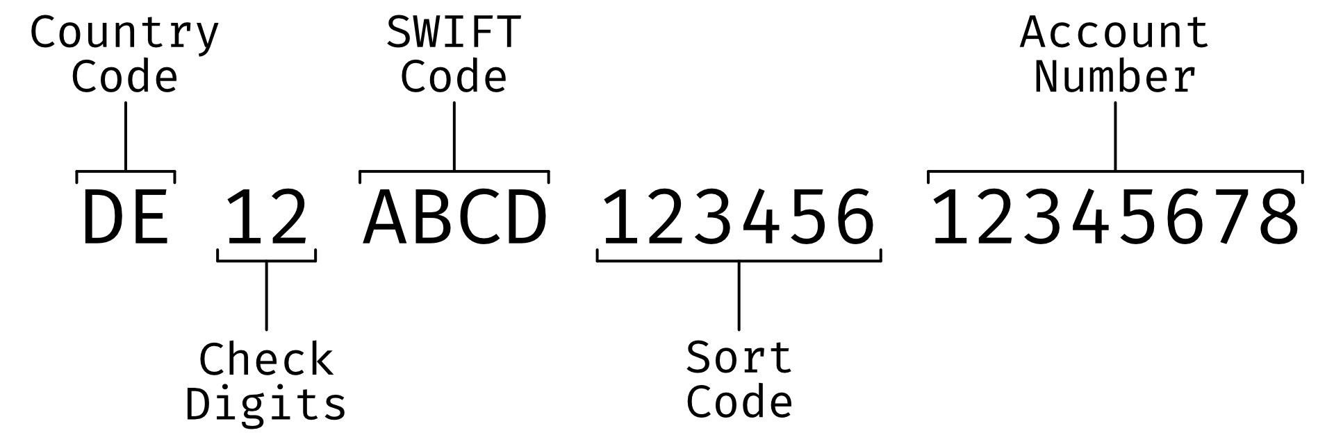
To get to that point, both datasets need to be combined somehow and then the IBAN needs to be generated out of the combined dataset. For more information see the original page: https://preppindata.blogspot.com/2023/01/2023-week-2-international-bank-account.html

The Solution

Like in the challenge of the first week, we will load the data using pandas' read_csv function and then we will look at the data itself.

import pandas as pd
transactions_df = pd.read_csv("Transactions.csv")
swift_code_df = pd.read_csv("Swift Codes.csv")
swift_code_df.head()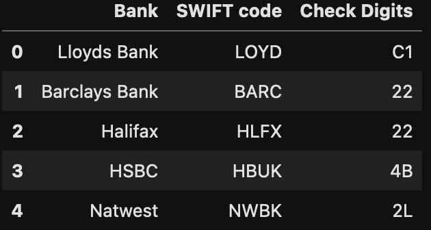

transactions_df.head()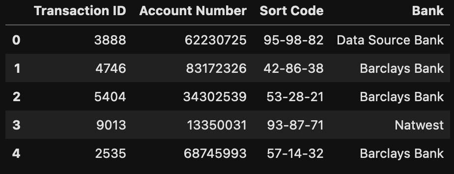

The first step that we need to do is to remove the dashes "-" in the Sort Code column, as they are not part of the IBAN. In order to do this, we will transform the column itself using string operations like this:

transactions_df["Sort Code"] = transactions_df["Sort Code"].apply(lambda x : x.replace("-", ""))
transactions_df.head()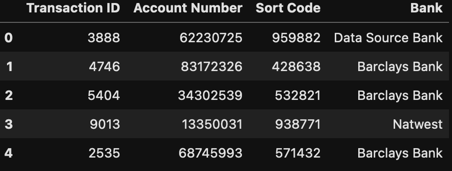

Then we need to create an additional column which contains the Country Code, which is currently missing and should contain "GB" on every row, as we are generating british IBANs in this challenge. This is done really fast using pandas DataFrames:

transactions_df["Country Code"] = "GB"
transactions_df.head()

The next step is probably the most complicated step to do, as we need to merge those two DataFrames together. But even for this pandas has the right solution which is the merge function. This allows us to perform SQL-JOIN-like operations using pandas DataFrames. For more information on this function have a look here: https://pandas.pydata.org/docs/reference/api/pandas.DataFrame.merge.html So in our case we would like to join the two DataFrames based on the Bank column which contains the name of the bank and is available in both DataFrames:

merged_df = pd.merge(transactions_df, swift_code_df, how="left", on="Bank")
merged_df.head()

Now we have all columns needed to generate the IBAN for each transaction. We just need to make sure that all columns we try to combine using the "+" operator are string-columns. This is why we need to transform them into a string first using the astype(str) method, if they could be numerical:

merged_df["IBAN"] = merged_df["Country Code"] + merged_df["Check Digits"].astype(str) + merged_df["SWIFT code"] + merged_df["Sort Code"].astype(str) + merged_df["Account Number"].astype(str)
merged_df.head()

Before we output the final table, we just need to remove all redundant columns, as most of the information are now available in the IBAN column. This is why all columns that we merged in the step before can be removed from the DataFrame:

merged_df = merged_df.drop(columns=["Account Number", "Sort Code", "SWIFT code", "Check Digits", "Country Code", "Bank"])
merged_df.head()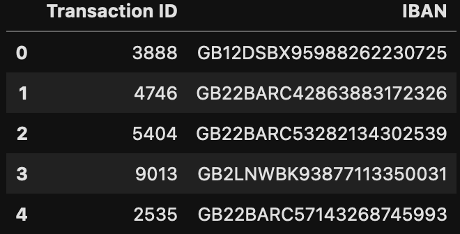

Now we just need to output the final DataFrame to complete the challenge:

merged_df.to_csv("Output.csv", index=False)

And if we combine all code-snippets from above we can complete the challenge with the following python script:

import pandas as pd
transactions_df = pd.read_csv("Transactions.csv")
swift_code_df = pd.read_csv("Swift Codes.csv")
transactions_df["Sort Code"] = transactions_df["Sort Code"].apply(lambda x : x.replace("-", ""))
transactions_df["Country Code"] = "GB"
merged_df = pd.merge(transactions_df, swift_code_df, how="left", on="Bank")
merged_df["IBAN"] = merged_df["Country Code"] + merged_df["Check Digits"].astype(str) + merged_df["SWIFT code"] + merged_df["Sort Code"].astype(str) + merged_df["Account Number"].astype(str)
merged_df = merged_df.drop(columns=["Account Number", "Sort Code", "SWIFT code", "Check Digits", "Country Code", "Bank"])
merged_df.to_csv("Output.csv", index=False)

Week 3

The Challenge

For the challenge in week 3 we will need to use the transaction file from week 1 again and we get a file with quarterly targets for each transaction type: Online and In-Person. To solve the challenge, we will need to compare target values for each transaction type in each quarter and to calculate the variance between the actual values and the target values. To do that we need to apply similar transformations as used in challenge for Week 1 on the transaction data, as well as to unpivot the given target data table. I will show what this means in detail in the solution part down below. For more information see the original channel posting: https://preppindata.blogspot.com/2023/01/2023-week-3-targets-for-dsb.html

The Solution

So firstly, as always, we need to import both csv files into pandas DataFrames and look on how the data is structured:

import pandas as pd
transactions_df = pd.read_csv("PD 2023 Wk 1 Input.csv")
targets_df = pd.read_csv("Targets.csv")
transactions_df.head()

targets_df.head()

As we can see right now the targets DataFrame has each quarter value in a separate column, which might be an issue later, as we will get one row per quarter from the transactions DataFrame. So a further step will require that we turn that columns into rows. But first let's transform the transaction DataFrame.

The first thing we need to do is to split the transaction code again to get the bank. This is necessary as we only want to calculate the summed-up values per quarter for the DSB bank. We first create the column bank where we extract the bank name from the transaction code into it and afterwards we filter our DataFrame to only contain rows where the bank column value is DSB.

transactions_df["Bank"] = transactions_df["Transaction Code"].apply(lambda x : x.split("-")[0])
transactions_df = transactions_df.loc[transactions_df["Bank"] == "DSB"]
transactions_df.head()

Then we encode the Online or In-Person column, so it contains text values instead of numerical ones, like we did for the challenge in week 1.

transactions_df["Online or In-Person"] = transactions_df["Online or In-Person"].replace({1 : "Online", 2: "In-Person"})
transactions_df.head()

Then again like in week 1, we need to parse and transform the Transaction Date. Therefore, we import the datetime library and parse the column with the strptime function. This time we do not want the day name, but instead we want to get the quarter from that date. Gladfully pandas gives has this built-in so we will just use that. For convenience reasons we can also rename the column from Transaction Date to Quarter, so we won't get confused later on.

import datetime
transactions_df["Transaction Date"] = transactions_df["Transaction Date"].apply(lambda x : datetime.datetime.strptime(x, "%d/%m/%Y %H:%M:%S"))
transactions_df["Transaction Date"] = transactions_df["Transaction Date"].dt.quarter
transactions_df = transactions_df.rename(columns={"Transaction Date": "Quarter"})
transactions_df.head()

Now it is time to sum the values by transaction type and quarter using the groupby function, which results in the following table:

summed_transactions_df = transactions_df[["Online or In-Person", "Quarter", "Value"]].groupby(["Online or In-Person", "Quarter"]).sum().reset_index()
summed_transactions_df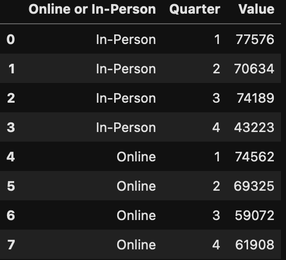

To achieve what we want we need to compare that table to the target values. But since both tables are not in the same format right now, we want to transform the targets DataFrame by performing an unpivot operation, which allows us to turn some of the column headings into row values, which looks somewhat like this:

Gladly pandas has a function for that, as this can be done using the melt function (more information see here: https://pandas.pydata.org/docs/reference/api/pandas.DataFrame.melt.html?highlight=melt#pandas.DataFrame.melt). So we are able to transform the targets DataFrame into our intended form by providing the quarter column names into the value_vars parameter of the function. Afterwards we can rename the resulting columns, so that the naming matches the column names of the transactions DataFrame. As the last transformation step, we just need to remove the letter Q from the quarter values as we only have numerical values in our transactions dataset and after that we are ready to merge both DataFrames together in order to compare target and actual values.

unpivot_transactions_df = pd.melt(targets_df, id_vars=["Online or In-Person"], value_vars=["Q1", "Q2", "Q3", "Q4"]).rename(columns={"variable": "Quarter", "value": "Value"})
unpivot_transactions_df["Quarter"] = unpivot_transactions_df["Quarter"].apply(lambda x : int(x[1:]))
unpivot_transactions_df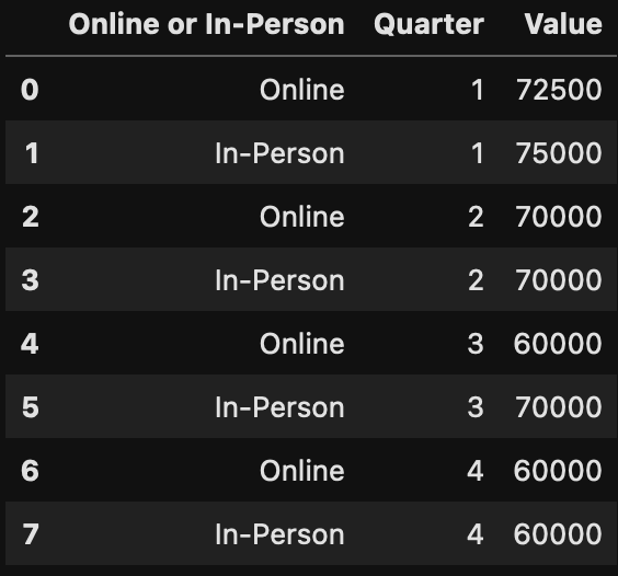

Merging those two DataFrames can be done using the merge function again. But this time we need to provide two keys, the transaction type, and the quarter, as neither of them has only unique values. After merging we then get the following DataFrame which gives us the basis for comparing the values.

merged_df = pd.merge(summed_transactions_df, unpivot_transactions_df, on=["Online or In-Person", "Quarter"], suffixes=(" Transactions", " Target"))
merged_df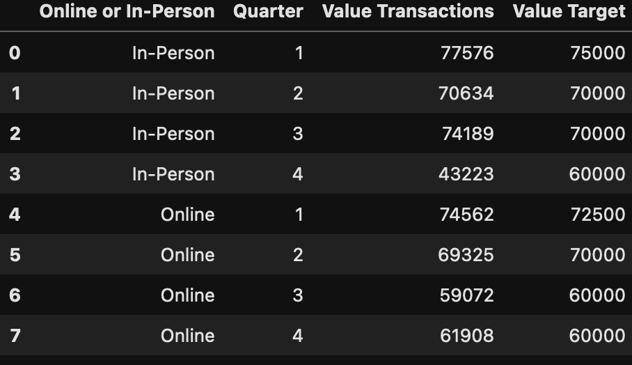

To calculate the difference, we now just need to calculate the difference between those two value columns and store them in a new column named Variance:

merged_df["Variance"] = merged_df["Value Transactions"] - merged_df["Value Target"]
merged_df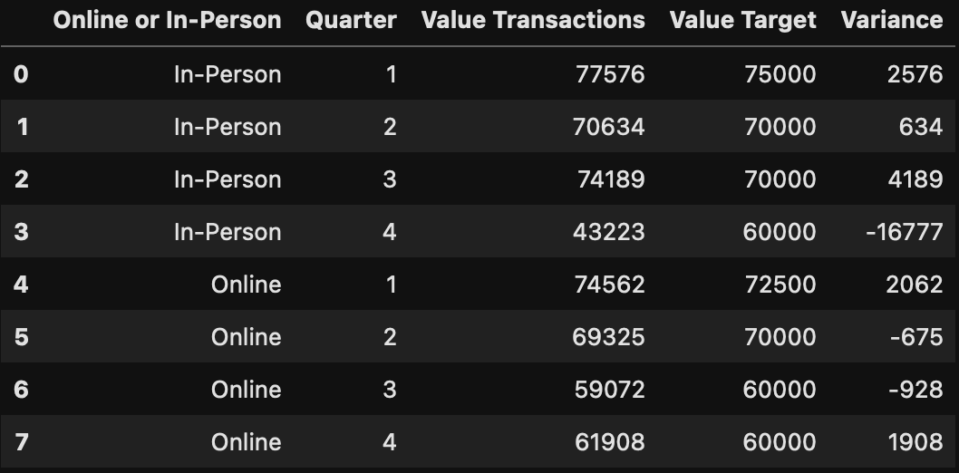

As always, the last step is to output our result into a csv file:

merged_df.to_csv("Output.csv", index=False)

Combining all code snippets together, we can solve the challenge with the following script:

import pandas as pd
import datetime
transactions_df = pd.read_csv("PD 2023 Wk 1 Input.csv")
targets_df = pd.read_csv("Targets.csv")
transactions_df["Bank"] = transactions_df["Transaction Code"].apply(lambda x : x.split("-")[0])
transactions_df = transactions_df.loc[transactions_df["Bank"] == "DSB"]
transactions_df["Online or In-Person"] = transactions_df["Online or In-Person"].replace({1 : "Online", 2: "In-Person"})
transactions_df["Transaction Date"] = transactions_df["Transaction Date"].apply(lambda x : datetime.datetime.strptime(x, "%d/%m/%Y %H:%M:%S"))
transactions_df["Transaction Date"] = transactions_df["Transaction Date"].dt.quarter
transactions_df = transactions_df.rename(columns={"Transaction Date": "Quarter"})
summed_transactions_df = transactions_df[["Online or In-Person", "Quarter", "Value"]].groupby(["Online or In-Person", "Quarter"]).sum().reset_index()
unpivot_transactions_df = pd.melt(targets_df, id_vars=["Online or In-Person"], value_vars=["Q1", "Q2", "Q3", "Q4"]).rename(columns={"variable": "Quarter", "value": "Value"})
unpivot_transactions_df["Quarter"] = unpivot_transactions_df["Quarter"].apply(lambda x : int(x[1:]))
merged_df = pd.merge(summed_transactions_df, unpivot_transactions_df, on=["Online or In-Person", "Quarter"], suffixes=(" Transactions", " Target"))
merged_df["Variance"] = merged_df["Value Transactions"] - merged_df["Value Target"]
merged_df.to_csv("Output.csv", index=False)

Week 4

The Challenge

For the last challenge in the introductory week of Preppin' Data, we get a trickier challenge to solve. The input file now consists of one Excel file which contains data of new customers instead of multiple csv files and additionally there are more than only one worksheet in that file. Each of those sheets contains 3 rows for each new customer in that specific month: One with the ethnicity, one with the date of birth and one with the account type. The fact that each of those values is in a separate row, instead of a column, makes it difficult to interpret the data and in addition to that, the column Demographic is misspelled in some of the sheets. The last difficulty of that challenge is, that there are some duplicate customer entries. But we will handle all of those problems in our solution.

For the original challenge information please refere here: https://preppindata.blogspot.com/2023/01/2023-week-4-new-customers.html

The Solution

We will start our solution like every other solution before by loading our data into a DataFrame. This time we will read 12 different DataFrames by passing the sheet index to the read_excel method. For each read sheet we will also create a column in the DataFrame named Month which stores the month number of the sheet. We will use this later, when we calculate the joining date of that customer, as we currently only have the joining day of that specific month sheet. After loading each month, we additionally combine all DataFrames by concatenating them on top of each other using the concat function.

import pandas as pd
arr = []
for i in range(12):
    month_df = pd.read_excel("New Customers.xlsx", sheet_name=i)
    month_df["Month"] = i + 1
    arr.append(month_df)
df = pd.concat(arr)
df.head()

As already mentioned in the introduction, some of the column names are misspelled, so the Demographic column exists in 3 different ways and shows up as 3 different columns in our DataFrame.

df[df["Demographic"].isna()]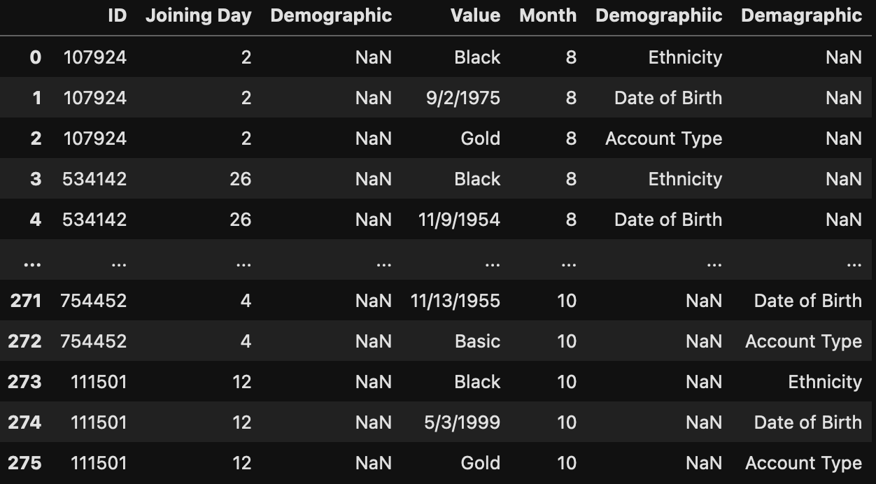

This is something we can resolve quick. We will fill the missing data in column Demographic using the fillna method, with the data in that row from column Demographiic and if after that there are still missing values, we will use column Demagraphic. After that both misspelled columns can be dropped, as we do not need them anymore.

df["Demographic"] = df["Demographic"].fillna(df["Demographiic"]).fillna(df["Demagraphic"])
df = df.drop(columns=["Demographiic", "Demagraphic"])
df.head()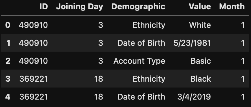

After dropping the additional columns, we can create our Joining Date column by creating a date object from the columns Joining Day, Month and the year 2023.

df["Joining Date"] = df[["Joining Day", "Month"]].apply(lambda x : datetime.date(2023, x["Month"], x["Joining Day"]), axis=1)
df.head()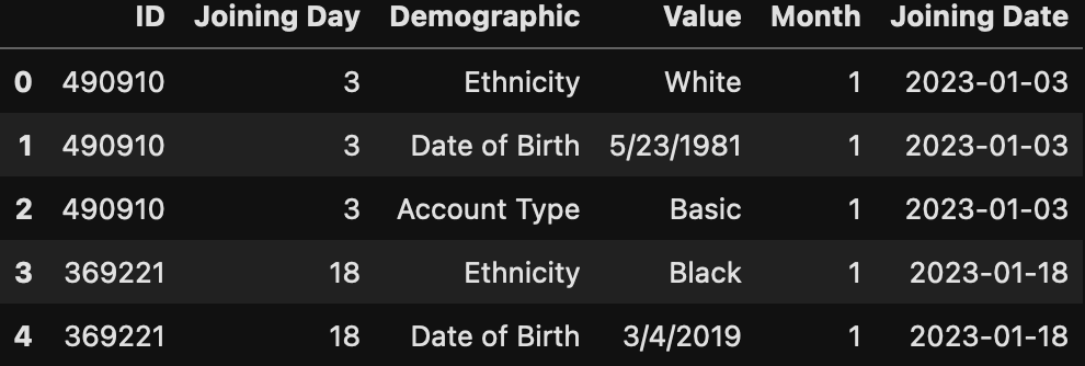

As there could be potential duplicates, we try to make a customer unique by creating a unique key which is simply a combination of the ID column and the Joining Date column. Everything under the assumption that a new customer should not appear on the same day twice. In larger datasets from real-world system this assumption may still be wrong and needs to be handled otherwise. But in our case this unique key is good enough.

df["Unique_Key"] = df["ID"].astype(str) + "_" + df["Joining Date"].astype(str)
df.head()

Once we have the unique key, we can finally use it in the pivot function to extract the data in the 3 customer rows into separate columns. If we wouldn't use the unique key we created and would use the ID column instead, pandas would throw an error because of duplicates, so this should be the way to go.

pivot_df = pd.pivot(df, index="Unique_Key", columns="Demographic", values="Value").reset_index()
pivot_df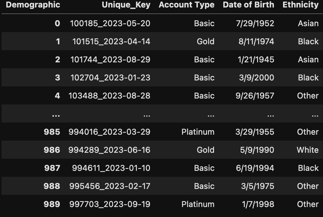

After creating our pivot table, we can join it back on our initial customer DataFrame. But as we don't need all columns from our initial DataFrame, we select only the columns we need, which are in our case Unique_Key, ID and Joining Date.

merged_df = pd.merge(df[["Unique_Key", "ID", "Joining Date"]], pivot_df, on="Unique_Key")
merged_df.head()

After the merge we have the problem, that for each customer now 3 rows which the exact same data exist. So, we only need to keep one of them and can drop the other 2 by using the drop_duplicates method in which we specify what our uniqueness attribute should be. Then we can also remove our unique key again as we do not need it anymore and that information also exist in other columns as well.

merged_df = merged_df.drop_duplicates("Unique_Key")
merged_df = merged_df.drop(columns="Unique_Key")
merged_df.head()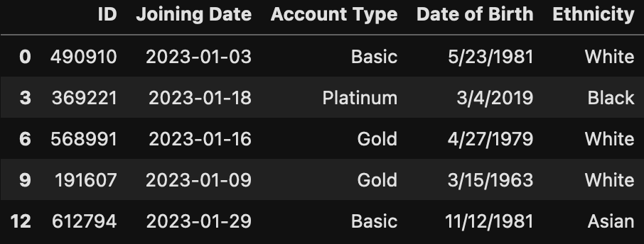

As an optional step, we can also convert the data in the Date of Birth column to a date object. This would make it convient to use that column in further analysis.

merged_df["Date of Birth"] = merged_df["Date of Birth"].apply(lambda x : datetime.datetime.strptime(x, "%m/%d/%Y").date())

Now we could work on our duplicate customer issue. When we take a look at the size of our DataFrame it shows that we have 990 rows in total.

merged_df.shape

When we now look at the number of unique values in the ID column, we can see that there are only 989 unique values. This shows us, that there is 1 customer entered twice in our data, so we need to remove that second entry from our DataFrame.

merged_df["ID"].unique().shape

To do that, we firstly sort our DataFrame by our Joining Date column in ascending order, so the earliest entry of our duplicate customer comes first in our DataFrame.

merged_df = merged_df.sort_values(by="Joining Date", ascending=True)
merged_df.head()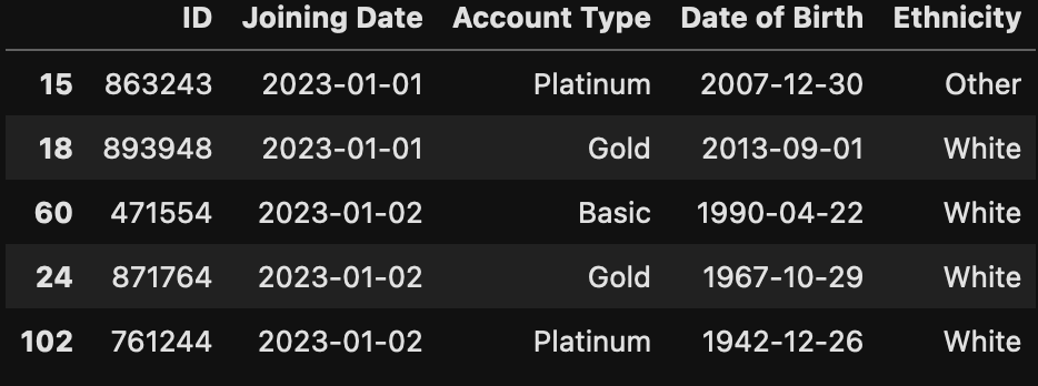

After that we can use the drop_duplicates method, which only keeps the first entry found of all duplicates, which is exactly what we want.

merged_df = merged_df.drop_duplicates("ID")
merged_df.head()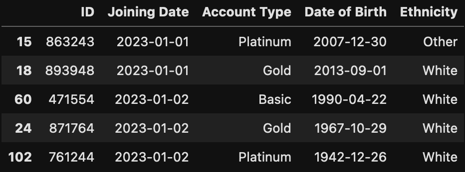

When looking at the size of our DataFrame now after removing that duplicated customer, we can see, that the size is now 989, so exactly the number of unique IDs in our DataFrame.

merged_df.shape

And last but not least, we output our result to a csv file:

merged_df.to_csv("Output.csv")

When we combine all code snippets from above, as for the previous challenges, we get the following code:

import pandas as pd
import datetime
arr = []
for i in range(12):
    month_df = pd.read_excel("New Customers.xlsx", sheet_name=i)
    month_df["Month"] = i + 1
    arr.append(month_df)
df = pd.concat(arr)
df["Demographic"] = df["Demographic"].fillna(df["Demographiic"]).fillna(df["Demagraphic"])
df = df.drop(columns=["Demographiic", "Demagraphic"])
df["Joining Date"] = df[["Joining Day", "Month"]].apply(lambda x : datetime.date(2023, x["Month"], x["Joining Day"]), axis=1)
df["Unique_Key"] = df["ID"].astype(str) + "\_" + df["Joining Date"].astype(str)
pivot_df = pd.pivot(df, index="Unique_Key", columns="Demographic", values="Value").reset_index()
merged_df = pd.merge(df[["Unique_Key", "ID", "Joining Date"]], pivot_df, on="Unique_Key")
merged_df = merged_df.drop_duplicates("Unique_Key")
merged_df = merged_df.drop(columns="Unique_Key")
merged_df["Date of Birth"] = merged_df["Date of Birth"].apply(lambda x : datetime.datetime.strptime(x, "%m/%d/%Y").date())
merged_df = merged_df.sort_values(by="Joining Date", ascending=True)
merged_df = merged_df.drop_duplicates("ID")
merged_df.to_csv("Output.csv")

Conclusion

To conclude this blog post of mine: The Preppin' Data challenges are a very good way to get into the whole data preparation space if you do not know where to start and I would highly recommend it to everyone that is currently just starting to get into the data field (like I am). In my opinion the last challenge was also of good complexity, and I am looking forward to complete upcoming challenges in the Intermediate and Advanced Month, and also subsequent challenges of course. Feel free to check out everything that is available on the Preppin' Data blog as well here: https://www.preppindata.com/